In this post, we will model and simulate an Ouster OS-1-64 in Gazebo, ROS’s simulation environment. Simulating the sensor in Gazebo allows users to experiment with the OS-1 sensor without needing to purchase the physical unit. Users can determine the ideal placement and orientation of the sensor for their specific application and evaluate the sensor’s performance when integrated into their robotics software stack. This ensures a smoother integration process when the user purchases an OS-1 and begins using it in their real-world applications. This post will cover the following topics:

• Developing an accurate URDF model of the sensor
• Rendering the sensor model in RViz and Gazebo
• Using Gazebo Laser plugins
• Publishing PointCloud2 messages with the correct structure

This work assumes the user is running Ubuntu 18.04 with ROS Melodic and Gazebo 9 installed.

Ouster OS-1 Overview

The OS-1-64 is a multi-beam flash lidar developed by Ouster. The sensor comes in 16 and 64 laser version. It’s capable of running at 10 or 20Hz and covers a full 360˚ in each scan. For horizontal resolution, the sensor support 512, 1024, or 2048 operating modes. The sensor has a 1m minimum range and a 150m maximum range. Finally, the sensor has an IMU onboard. For more detailed specifications of the sensor, refer to the OS-1 Product Page.

On the software side, Ouster provides sample code for connecting to and configuring the OS-1, reading and visualizing data, and interfacing with ROS. Specifically, the ouster_ros package contains sample code for publishing OS-1 data as standard ROS topics. The package contains the following ROS nodes:

• os1_node: The primary sensor client that handles the sensor initialization and configuration as well as publishing the raw IMU and lidar packets
• os1_cloud_node: Converts the raw IMU and lidar packets to ROS IMU and PointCloud2 messages
• viz_node: Runs the provided visualizer displaying the pointcloud and the intensity/noise/range images
• img_node: Publishes the intensity/noise/range images as ROS image messages

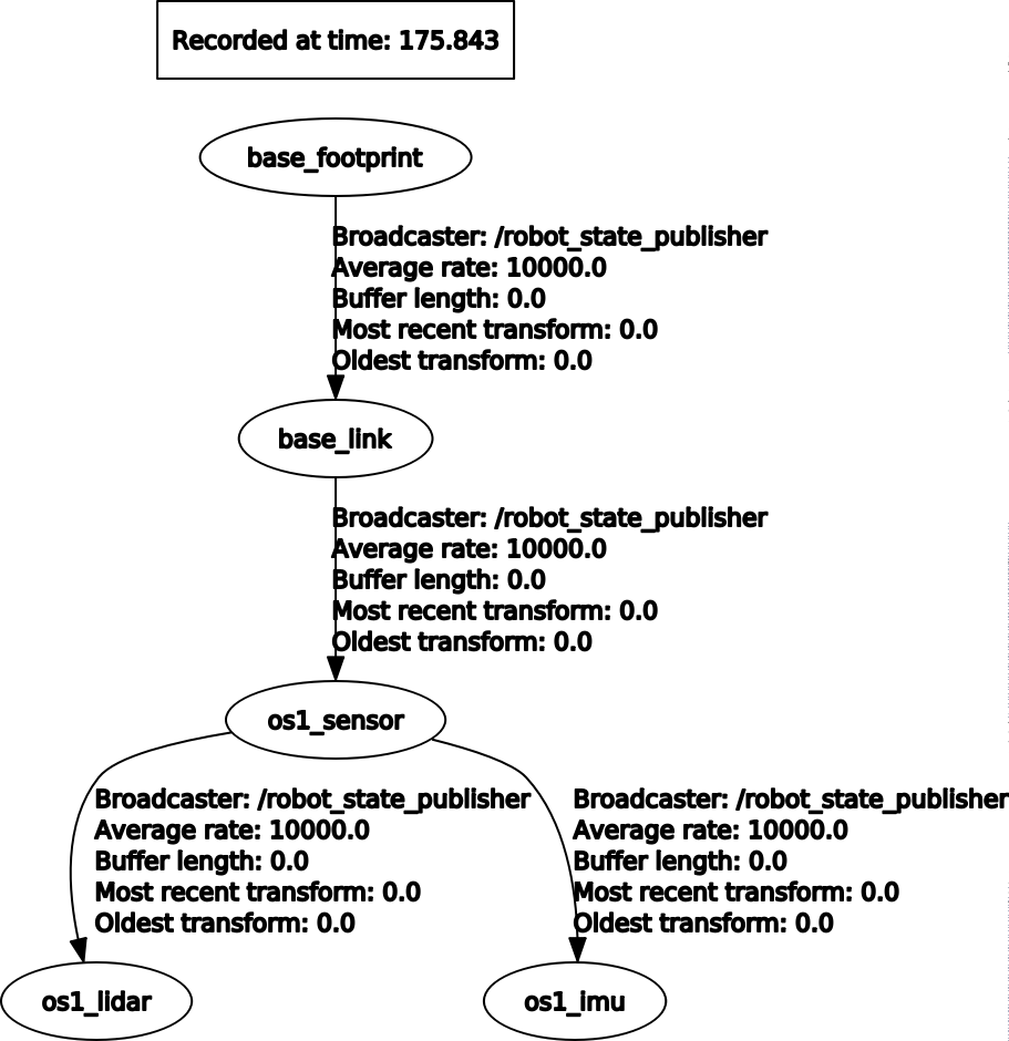
The sensor also publishes TF transforms between the lidar and IMU coordinate frames. These are shown in the TF tree below:

The provided sample data can be replayed through the ROS driver to produce the ROS topics and TF tree discussed above. This is done by running the following command:

$ roslaunch ouster_ros os1.launch replay:=true viz:=true image:=true

The resulting data can be viewed in both RViz and the provided visualizer.

The goal of this project is to accurately mimic the physical properties of the OS-1 sensor and publish simulated data using the same ROS messages.

Create the SDF Model

SDF is an XML format that describes objects and environments for robot simulators, visualization, and control. For this project, we will be using a fork of the ouster_example code. The SDF model will be created in a .world file that can be visualized in Gazebo.

The first step is to define the link property which includes the inertial and collision fields. These values are based on the physical dimensions of the OS-1 sensor. We can reference the datasheet to determine the sensor dimensions.

From the datasheet, we collect and input the following parameters:

• Mass: 380g
• Height: 73mm
• Diameter: 84mm

The moment of inertia matrix can be computed using equations found on Wikipedia. These are input into the appropriate fields in the OS1-64.urdf.xacro file.

The model can now be visualized in Gazebo for debugging.

$ gazebo os-1-64.world -u

When gazebo loads, you will see the <visual> elements of the model, which define how a model looks. The <collision> elements, on the other hand, define how the model will behave when colliding with other models. To see, and debug, the <collision> elements right-click on a model and choose View->Collisions.

It’s also possible to visualize the inertia values. With Gazebo running, right-click on the sensor and select View->Inertia. This will cause a purple box to appear.

Next, we want to add 3D meshes to make the sensor look more realistic. Gazebo can only use STL, OBJ or Collada files, so you may need to convert your file to one of these formats. The Gazebo tutorials provide an example of this conversion process using FreeCad. The mesh file we will use is provided in the ouster_description package named os1_64.dae.

To use this mesh file, update the <visual> element and replace the <cylinder> element within with a <mesh> element. The <mesh> element should have a child <uri> that points to the top collada visual. The resulting model is shown below in RViz and Gazebo.

Create the URDF Model

Now that we have the basic dimensions and visual appearance rendered correctly, we can add the simulated IMU and lidar sensors. We take the core components from the SDF model and convert them to the OS1-64.urdf.xacro model.

The Universal Robotic Description Format (URDF) is an XML file format used in ROS to describe all elements of a robot. To use a URDF file in Gazebo, some additional simulation-specific tags must be added to work properly with Gazebo. We use Xacro (XML Macros) and with the macro tag, specify the macro name and the list of parameters. The list of parameters become macro-local properties.

First, we add links for the IMU and lidar sensor. These are required to match the TF tree published by the real sensor. These frames contain the transformations between the IMU sensor and the lidar sensor. These links are named “os1_imu” and “os1_lidar” and connected to the parent link, “os1_sensor” through the “imu_link_joint” and the “lidar_joint_link”.

The last major joint element to add is a joint between the sensor and the object it is attached to. We assume that the sensor will be rigidly affixed to the robot. We create the <joint> property using a fixed joint between the OS-1 and its parent frame named “mount_joint”.

It’s possible to visualize joints for debugging purposes. With Gazebo running, Right-click on a model, and choose View->Joints. Joints are often located within a model, so you may have to make a model transparent to see the joint visualization (Right-click on the model and select View->Transparent).

Add the Sensor to the Model

A sensor is used to generate data from the environment or a model. In this section, we will adapt Dataspeed Inc’s velodyne_simulator package to support the OS-1. This plugin is based on the gazebo_plugins/gazebo_ros_block_laser plugin. We will again reference the datasheet for the following properties:

• Lasers
• Horizontal Resolution
• Field of View
• Minimum and Maximum Range
• Range Resolution

Given this information, the plugin element is added. This references the libgazebo_ros_ouster_laser.so plugin generated by the files in the ouster_gazebo_plugins package. This plugin published lidar data using the PointCloud2 message format on the /os1_cloud_node/points topic.

The OS-1 also contains an IMU. We use the hector_gazebo_plugins package to simulate the IMU sensor. We add a plugin element referencing the libhector_gazebo_ros_imu.so plugin. This plugin publishes IMU data on the /os1_cloud_node/imu topic.

Finally, we want to enable the user to easily change the configuration of the simulated sensor. The following parameters are configurable through the xacro macro:

• origin
• parent (default = base_link)
• name (default = os1_sensor)
• topic (default = /os1_cloud_node/points)
• hz (default =10)
• lasers (default = 64)
• samples (default =512)
• min_range (default = 0.9)
• max_range (default = 75.0)
• noise (default = 0.008)
• min_angle (default = -PI)
• max_angle (default = PI)

Visualizing the Sensor

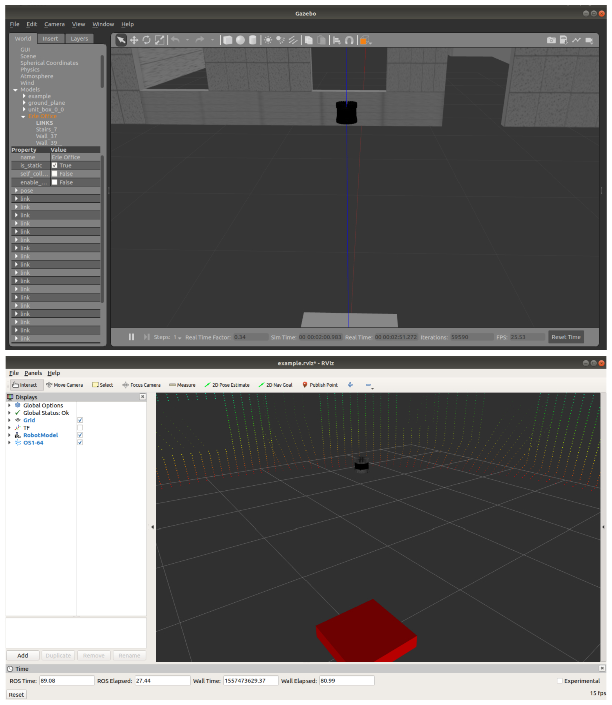
Once the simulated sensor is properly configured, it’s possible to visualize the output. We can use a launch file to load the OS-1 model into a Gazebo environment and launch RViz. This is the purpose of the os1_world.launch  file. When this file is run, the example.world and example.urdf.xacro files are loaded.

The example.world file loads a Gazebo environment with the Erle office model. The example.urdf.xacro creates a base box and attaches the OS-1 above it. The launch file is executed by running the command:

$ roslaunch ouster_description os1_world.launch

The images below show the model visualized in Gazebo as well as RViz. RViz displays the points as well as the coordinate frames for each TF which is helpful for debugging purposes.

You can verify that the model is outputting the IMU and PointCloud2 messages as expected by running:

$ rostopic hz /os1_cloud_node/{imu,points}

You can also verify the TF tree by running:

$ rosrun tf view_frames

which outputs an image depicting the TF tree:

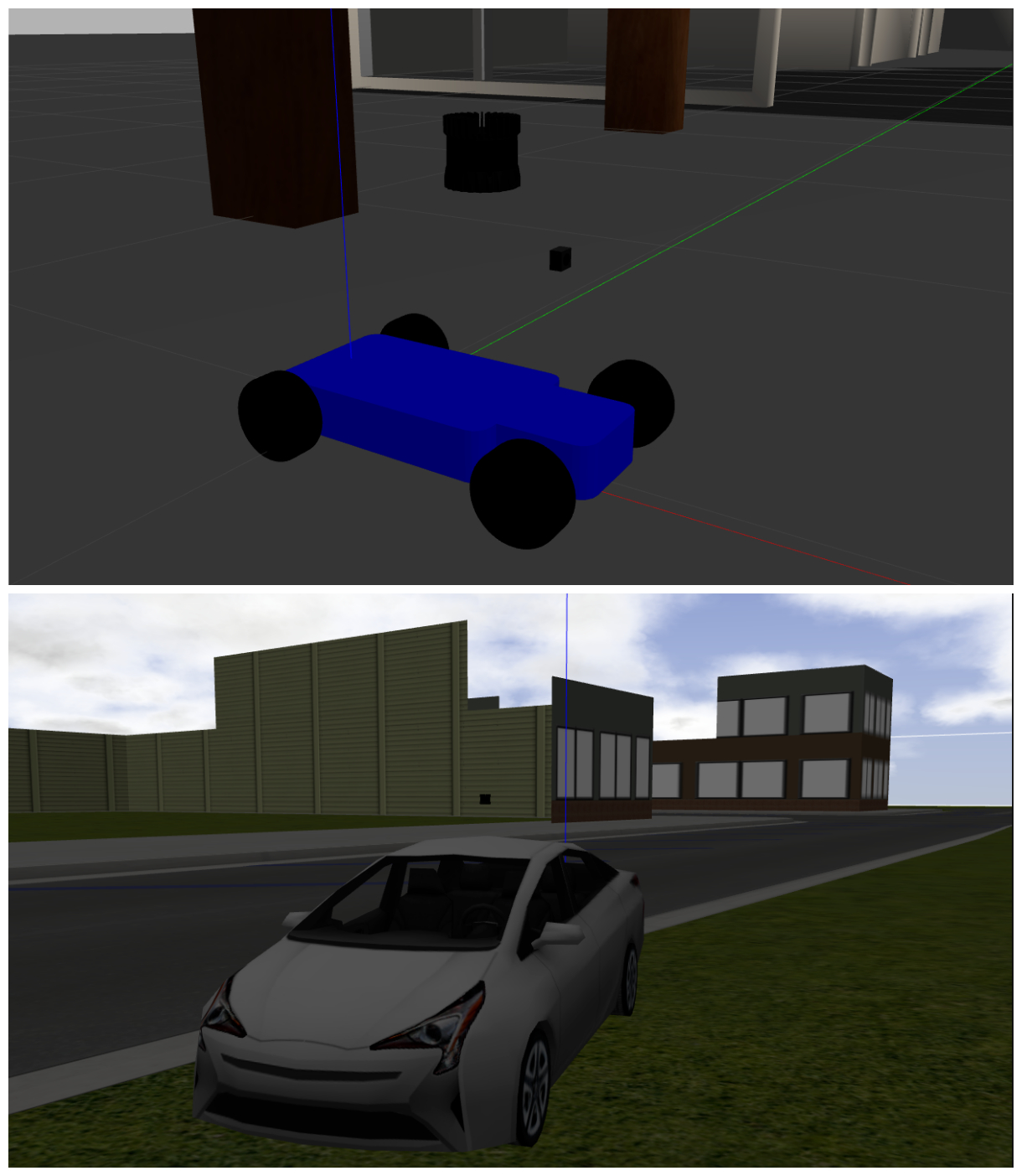
Since the OS-1 is configured using xacro URDF, it can easily be attached to other robots for simulations. The image below shows the OS-1 simulated on an RC car as well as a Prius.