Below are some of my key takeaways from reading the book, Thinking in Systems, by Donella H. Meadows. If you are interested in more detailed notes from this book, they are available here.
Below are some of my key takeaways from reading the book, Thinking in Systems, by Donella H. Meadows. If you are interested in more detailed notes from this book, they are available here.
In 2020, I was given the opportunity to lead the Product team at Ouster. This post details the process and framework I used to define the core functions of the team and figure out where to start.
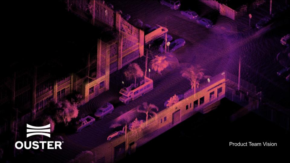
Ouster’s core business is the design and manufacture of high-resolution lidar sensors supporting a wide variety of robotics applications. As a result of the unique digital lidar architecture taken at Ouster, we’re able to develop lidar systems that are smaller, lighter, and less expensive without sacrificing on core performance. Ouster currently has 600 customers and recently launched it’s second generation lidar sensors. The product offering expanded beyond the original OS1 lidar sensor to include the OS0, optimized for short range performance, and the OS2, which supports applications regarding longer ranges.
Below are some of my key takeaways from reading the book, The Sovereign Individual by James Davidson and Lord William Rees-Mogg. If you are interested in more detailed notes from this book, they are available here.

Below are some of my key takeaways from reading the book, The Beginning of Infinity by David Deutsch. If you are interested in more detailed notes from this book, they are available here.
In November of 2018, Amazon announced the launch of RoboMaker, a cloud robotics service that makes it easy to develop, simulate, and deploy robotics applications at scale. RoboMaker provides a robotics development environment for application development, a robotics simulation service to accelerate application testing, and a robotics fleet management service for remote application deployment, update, and management.
RoboMaker extends the Robot Operating System (ROS) with connectivity to cloud services and integrations with various Amazon and AWS services. This makes it easy to integrate machine learning, voice recognition, and language processing capabilities with the robotics application. RoboMaker provides extensions for cloud services like Amazon Kinesis (video streams), Amazon Rekognition (image and video analysis), Amazon Lex (speech recognition), Amazon Polly (speech generation), and Amazon CloudWatch (logging and monitoring) to developers who are using ROS.
In this example, the code base used to simulate an RC car and Ouster OS1 lidar sensor in Gazebo and Rviz is modified to support continued development and simulation via AWS RoboMaker.
A friend of mine was asking me about the technical complexity of a children’s picture book reading robot, the Luka. The robot is used to read children’s books in both English and Chinese. It looks at the pages and then reads the book aloud in English or Chinese.

This product has three primary requirements:
As a proof of concept, I used the following image as an example use case.

I leveraged several APIs to replicate the functionality. The sample code is available here in a Google Colab notebook.
Below are some of my key takeaways from reading the book, The Practicing Stoic: A Philosophical User’s Manual by Ward Farnsworth. If you are interested in more detailed notes from this book, they are available here.

The planning fallacy, first proposed by Daniel Kahneman and Amos Tversky in 1979, describes a bias that causes people to underestimate how long something will take and overestimate its impact. As a Product Manager, this is disheartening to read, but also not surprising. Features take longer to release than anticipated and they rarely deliver the maximum value to the user on the first release. Uncertainty internal to the organization makes it difficult to accurately estimate development timelines. Uncertainty external to the organization makes it difficult to gauge the impact of features. We need to develop tools that embrace uncertainty so we can mitigate the effects of the planning fallacy and remain flexible to the realities of an uncertain future.
Below are some of my key takeaways from reading the book, Making Things Happen by Scott Berkun. If you are interested in more detailed notes from this book, they are available here.