This section describes the development and implementation of an image segmentation algorithm to identify and track lanes in an image. This work was inspired by the Udacity Self Driving Car Engineer Nanodegree program. This work references the open-source projects of some of the students who completed the Basic Lane Detection and the Advanced Lane Detection projects.
Required Dependencies
This project leverages the OpenCV (Open Source Computer Vision Library) libraries to implement a range of image processing algorithms. OpenCV was designed for computational efficiency and with a strong focus on real-time applications. Written in optimized C/C++, the library can take advantage of multi-core processing. To verify that OpenCV is installed, run the following commands:
$ python
>>> import cv2
>>> cv2.__version__
'2.4.9.1'
>>>
ROS also provides the vision_opencv stack which packages the OpenCV library for ROS. This stack provides the cv_bridge and image_geometry packages. The cv_bridge package serves as the interface between OpenCV image variables and ROS image messages.
Camera Calibration
The raspicam_node package contains a calibration file for the RaspberryPi camera. However, it is suggested to recalibrate the camera if you are using a non-default image size. Since this project resizes the image to a 320×240 image to improve processing speed, it was necessary to re-calibrate the camera.
A camera calibration can be run with the following commands. These need to be updated based on the size and dimensions of the checkerboard you use.
$ roslaunch raspicam_node camerav2_320x240.launch
$ rosrun image_transport republish compressed in:=/raspicam_node/image raw out:=/raspicam_node/image
$ rosrun camera_calibration cameracalibrator.py --size 8x6 --square 0.74 image:=/raspicam_node/image camera:=/raspicam_node
Save the camera calibration file in the camera_info directory of the raspicam_node package and update the camerav2_320x240.launch file to ensure the calibration file is loaded.
Image Segmentation Algorithm
Relying on the OpenCV library, the lane_detection package contains the nodes and functions to support lane detection and tracking. For this project, we will focus on identifying the center lane and providing the position of the lane to a control algorithm. The control algorithm then computes the desired velocities required to keep the autonomous car centered on the lane.
The algorithm begins by receiving a raw image from the RaspberryPi camera. For the purposes of this walk through, we will use an image from the Conde Gazebo world described in the Drive-by-Wire Development section. The basic image segmentation and processing functions are defined in the lane_detection_module.py file.
The first step in the algorithm is to apply a mask to the image. This mask keeps the region of the image defined by the given polygon, defined by the vertices variable, and sets the rest of the image black. Since we know that the lane lines will likely be in the center of the image, we can use the mask to remove any objects that might match the color of the lanes but are not our desired target. The masking is performed by the region_of_interest function.
def region_of_interest(img, vertices):

    #defining a blank mask to start with
    mask = np.zeros_like(img)

    #defining a 3 channel or 1 channel color to fill the mask with depending on the input image
    if len(img.shape) > 2:
        channel_count = img.shape[2]  # i.e. 3 or 4 depending on your image
        ignore_mask_color = (255,) * channel_count
    else:
        ignore_mask_color = 255

    #filling pixels inside the polygon defined by "vertices" with the fill color
    cv2.fillPoly(mask, vertices, ignore_mask_color)

    #returning the image only where mask pixels are nonzero
    masked_image = cv2.bitwise_and(img, mask)
return masked_image
This function returns a masked image.
Next, a perspective transform is performed on the masked image to create a warped image. The perspective_transform function transforms the image from the front-facing camera view to a top down “bird’s-eye” view. The front-facing camera view’s perspective distortion causes parallel, straight lanes to converge at a vanishing point. This transformation makes the processing easier for the lane detection algorithms since parallel, straight lines are rendered as vertical lines.
def perspective_transform(image, corners, xoffset=0):

     height, width = image.shape[0:2]
     output_size = height/2

     new_top_left=np.array([corners[0,0],0])
     new_top_right=np.array([corners[3,0],0])
     offset=[xoffset,0]
     img_size = (image.shape[1], image.shape[0])
     src = np.float32([corners[0],corners[1],corners[2],corners[3]])
     dst = np.float32([corners[0]+offset,new_top_left+offset,new_top_right-offset ,corners[3]-offset])

     M = cv2.getPerspectiveTransform(src, dst)

     warped = cv2.warpPerspective(image, M, (width, height), flags=cv2.INTER_LINEAR)

return warped, src, dst
The perspective transform requires arrays of source and destination points. The goal is to have a warped image with vertical lines. The source and destination points can be determined by manually inspecting an image with known parallel lines as shown below. The series of images below depicts the transformation with the source and destination points identified.
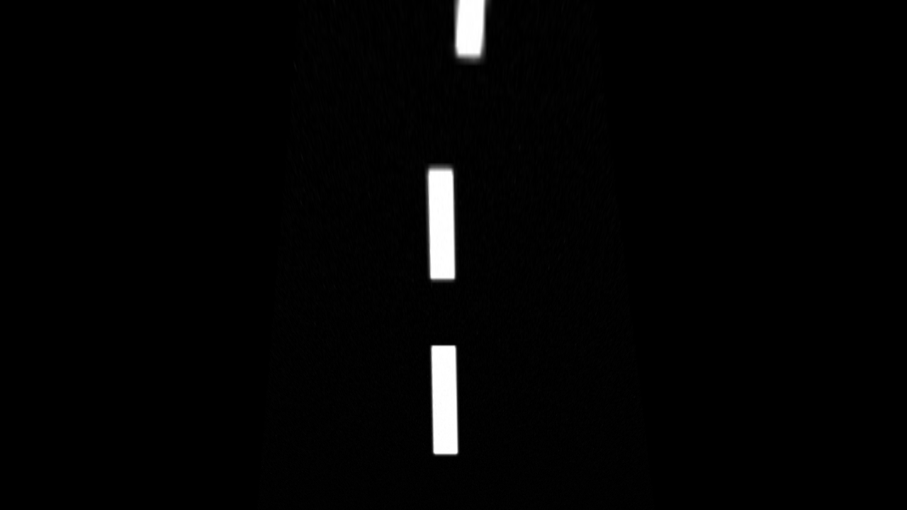
Once the source and destination points are determined, the transformation can be applied to the images in the pipeline. The image below is an example of the warped output image.
The next step is to take the warped image and identify pixels that are likely to be the lanes. This will in a binary image, with the pixels that met the criteria set as white and the remaining pixels set to black. For this initial implementation, basic thresholding was used. The inputs to the binary_thresh function are an image and a series of minimum and maximum values for each channel in the image.
def binary_thresh( img,  boundaries,  filter):

     if filter == 'RGB':
         frame_to_thresh = img.copy()
     else:
         frame_to_thresh = cv2.cvtColor(img, cv2.COLOR_BGR2HSV)

     for (lower,  upper) in boundaries:

         # create numpy arrays from the boundaries
         lower = np.array(lower,  dtype = "uint8")
         upper = np.array(upper,  dtype = "uint8")

         # find the colors within the specified boundaries and apply the mask
         mask = cv2.inRange(frame_to_thresh,  lower,  upper)
         output = cv2.bitwise_and(frame_to_thresh, frame_to_thresh,  mask = mask)   #Returns an RGB image

return mask
The thresholds can be determined by examining a series of images under varying lighting conditions and identifying the optimal thresholds for each channel that result in a binary image where the lane is detected without additional noise. This process is described in more detail in subsequent sections. An example output image is below.
Once the image has been segmented, ideally with the lane detected, we need to calculate the position of the lane. The position of the lane is estimated by fitting a polynomial line to the lane pixels. This process is performed by the fit_polynomials function which is available in the lane_detection_module.py fie for further review. In general, the function performs the following steps:
- Calculates a histogram of the bottom half of the image
- Find the peak of that histogram
- Partition the image into horizontal windows
- Start the bottom window at the peak of the histogram, assuming this is the lane
- Move up the image to find pixels that are likely to be part of the lane, re-centering the sliding windows opportunistically
- Fit a polynomial to the group of pixels, which represents the estimated lane line
A visualization of this process is shown below.
For debugging purposes, it is helpful to visualize the output of this process on the original image. The pixels identified as lane pixels are highlighted and the line fitting the lane pixels are both displayed on top of the original image.
Simulation
The Gazebo simulator is perfect for testing the image processing and control systems design. The Conde Gazebo world described in the Drive-by-Wire Development section is useful for this purpose. The goal of this simulation is to identify and track the center lane around the “figure eight” track.
The nodegraph below shows the nodes and topics required for this simulation. In contrast to the drive-by-wire set-up, we now have multiple control commands being computed and combined in the yocs_cmd_vel_mux node. The center_line_detection node is responsible for performing the image segmentation and computing the desired trajectories based on the position of the lane identified in the image.
The center_line_detection node subscribes and publishes on several topics.
"""ROS Subscriptions """
self.image_sub = rospy.Subscriber("/raspicam_node/image/image_raw",Image,self.cvt_image)

self.image_pub = rospy.Publisher("/image_converter/output_video",Image, queue_size=10)
self.cmdVelocityPub = rospy.Publisher('/platform_control/cmd_vel', Twist, queue_size=10)
self.cmdVelocityStampedPub = rospy.Publisher('/platform_control/cmd_vel_stamped', TwistStamped, queue_size=10)
The node receives images from the camera and outputs a processed image. The node also computes the desired speeds and publishes those commands with and without a timestamp.
Once an image is received, the image goes through the segmentation process identified above.
# apply ROI mask
self.maskedImage = ld.region_of_interest(self.latestImage, self.vertices)

# perspective transform
self.warpedImage,  _,  _ = ld.perspective_transform(self.maskedImage, self.corners)

# detect binary lane markings
self.binaryImage = ld.binary_thresh(self.warpedImage, self.boundaries, 'HSV') #RGB or HSV
Given the segmented image, the node computes the line of best fit for the lane. If detected, the line is drawn on the output image.
# it polynomials
if self.global_fit is not None:
    ploty, fitx, fit = ld.fast_fit_polynomials(self.binaryImage,  self.global_fit)
else:
    ploty, fitx, fit = ld.fit_polynomials(self.warpedImage, self.binaryImage)

self.global_fit = fit

# draw lane
self.processedImage = ld.render_lane(self.maskedRGBImage, self.corners, ploty, fitx)
Given the line of best fit for the detected lane, the point where the line crosses the bottom of the image is used as the setpoint for the control algorithm. The goal of the control algorithm is to compute the desired speeds to keep this setpoint at the center of the image. A simple moving average is used to smooth out the calculation of the setpoint and reduce the impact of outliers.
# Calculate Setpoint
pts = np.vstack((fitx,ploty)).astype(np.float64).T
self.avg = ld.movingAverage(self.avg, pts[-1][0],  N=3)
self.intersectionPoint = np.array([self.avg])

# Adjust Motors
self.flag = control.adjustMotorSpeed(self.latestImage,  self.intersectionPoint,  self.speed,  self.cmdVelocityPub, self.cmdVelocityStampedPub, self.flag)

# Publish Processed Image
self.outputImage = self.processedImage
self.publish(self.outputImage, self.bridge, self.image_pub)
Once the desired velocities are computed and published, the output image is published and the process repeats on the latest image
The center_line_detection node computes desired velocities and publishes them on the /platform_control/cmd_vel topic. This is the topic reserved for autonomous navigation commands. The yocs_cmd_vel_mux node receives these commands and computes the final speed commands. For the simulation, these commands are sent to Gazebo to maneuver the simulated vehicle. An image from a simulation is shown below.
Software-in-the-loop Simulations
The Gazebo simulator is good for debugging the image segmentation algorithm and verifying the system architecture with the correct nodes and topics. The next step is to verify the image segmentation algorithm and control system on real-world data. This is called a software-in-the-loop simulation.
First, we need to manually drive the vehicle around the test track and record data. Specifically the images and control commands are recorded. Make sure the record_cam flag is set to “true” in rover_dbw_cam.launch and launch the file.
$ roslaunch rover_teleop rover_dbw_cam.launch
Manually drive the vehicle around the track for at least one complete lap and make sure a new rosbag file is recorded in the data/ folder in the rover_teleop package.
Next, we will refine the bag file. First we will trim the bag file to remove any unwanted data. This can be done by playing the file and viewing the images in rqt_image_view.
$ rosbag play <filename>
$ rqt_image_view
Record the beginning and ending time of the data you want to keep. The times are displayed in the terminal where the bag file is being played.
Next, filter the bag so that only the image and velocity command topics are in the bag. Then trim the bag file down based on the start and stop times recorded earlier. Modify the commands based on your times and filenames.
$ rosbag filter <original.bag> <output1.bag> "'topic=/raspicam_node/image/compressed' or topic='/joy_teleop/cmd_vel_stamped'"
$ rosbag filter <output1.bag> <processed.bag> "t.to_sec() >= <start time>" "t.to_sec() <= <end time>"
The next step is to determine the best threshold values for identifying the lane lines. Now that the bag file has been refined, save a couple example images. Play the bag file, run the rqt image viewer, and save some images using the image viewer.
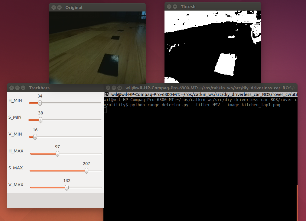
provides a series of image processing utilities. One function, range-detector, allows the user to threshold each channel of an RGB or HSV image and preview the result in real-time. Run this script on each of the sample photos and try to determine the best values for each channel. The resulting image should have the lane lines detected while limiting noise and other objects as much as possible. Remember that the image processing pipeline will remove portions of the image outside the specified region of interest so don’t be too concerned with false positives outside the ROI. Run the program using the following command in the directory where you saved the range-detector file.
$ python range-detector.py --filter HSV --image <file.png>
For this implementation, the images are converted to HSV format for segmentation instead of RGB. Unlike RBG, HSV separates the color components from the intensity. This makes it more robust to lighting changes and more effective for our purposes.
The center_line_detection node file needs to be updated with several environment and camera specific variables including the threshold values. Find an image from the bag file where the vehicle is centered between parallel lines or run rover_dbw_cam.launch again and save an image. Record points along the parallel lines that can be used as source points for the perspective transformation. Save these points as self.corners.
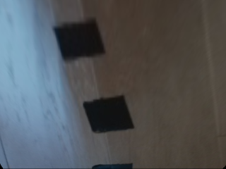
 This transformation results in a warped image as shown below.
Based on your environment, establish your desired region of interest used to create the image mask. Save these points as self.vertices .
Lastly, enter the threshold values as self.boundaries .
We will use a modified launch file, rover_center_line_cam_hitl.launch, to view the output of our image segmentation algorithm and control calculations. This launch file plays the refined bag file as well as the nodes required for autonomous navigation. It does not run the rosserial node required for connecting to the Arduino since this isn’t required for this test.
First we want to test our threshold values. Sometimes this is easier without the mask. Make the following changes in center_line_detection node.py to view the image segmentation on the original image.
--- self.binaryImage = ld.binary_thresh(self.warpedImage, self.boundaries, 'HSV')
+++ self.binaryImage = ld.binary_thresh(self.latestImage, self.boundaries, 'HSV')

--- self.outputImage = self.processedImage
+++ self.outputImage = self.maskedRGBImage
Launch rover_center_line_cam_hitl.launch to view the performance of the image segmentation algorithm on the entire bag file. If you find problem areas, save an image and evaluate it using the range_detector.py script. Adjust your threshold values until you get the most reliable performance.
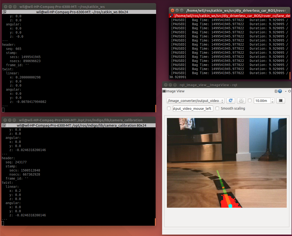
Undo the changes to the code so center_line_detection node.py is back in its original form. This time, we will view the lane detection with the line of best fit visualized. The line should display consistently as long as the lane segments are detected. The blue dot shows the setpoint position that will be sent to the controller. Adjust the ld.movingAverage window to improve the responsiveness of the setpoint calculation.
Lastly, we will compare the computed velocities with the velocities recorded when manually driving the track. This will help us ensure that the control system is calculating realistic numbers before running on the real system. Run rover_center_line_cam_hitl.launch again while monitoring the recorded commands on the “/joy_teleop/cmd_vel” topic and the computed commands on the “/platform_control/cmd_vel” topic.
Once satisfied with the performance of the image segmentation algorithm and the control system, it is time to test everything on the real vehicle.
Real World Implementation
The final test uses the entire software suite to autonomously navigate the Elegoo car around the track without any user input. I use the Tempus Monitor and Integrated Keyboard to connect to the RaspberryPi.
Before starting the lane detection program, make sure the Elegoo power source is powered off. Also, make sure the Xbox controller is running, connected, and you can see the output as described in the Raspberry Pi Integration section. Lastly, ensure that the Arduino is running the rover_motors.ino sketch, detailed in the Drive-by-Wire Development section.
Start the lane detection program using the following command to launch rover_center_line_cam.launch.
$roslaunch lane_detection rover_center_line_cam.launch
This launch file results in the rosgraph shown below.
Once the system is up and running, connect to the RaspberryPi from a remote computer using the tightvncserver on the RaspberryPi as described in the Raspberry Pi Integration section. Start rwt_image_viewer to monitor the output of the image processing algorithm. Once you are satisfied that everything is functioning properly, turn on the power source on the Elegoo. The motors should begin receiving commands and moving the vehicle. If the vehicle begins to move off track, you can manually override the autonomy commands with the Xbox controller.
The video below provides a quick summary of this section including the Elegoo navigating autonomously around a track with a black center lane line.
[embedyt] https://www.youtube.com/watch?v=zrk9qAqG2o4%5B/embedyt%5D


